Signal Generation, Transmission, and Reception
In the process of IoT network construction and data transmission, various wireless signals are inevitably encountered—among which electromagnetic signals and acoustic (sound) waves are two representative types. To realize the fundamental functions of wireless transmission—and the advanced technologies built upon them—we must first understand basic signal processing methods and related theoretical knowledge, preferably complemented by hands-on experimentation.
In real-world scenarios, electromagnetic waves are predominantly used for communication and sensing. Fortunately, commercially available devices now enable practical signal processing—for example, Universal Software Radio Peripheral (USRP) devices can process electromagnetic wave signals.
To help learners intuitively experience and study signal characteristics—and to make signals visually observable and directly analyzable—the remainder of this course (unless otherwise specified) will use acoustic signals to simulate various IoT connectivity techniques. This approach offers several advantages:
- Acoustic signals effectively emulate key properties of electromagnetic waves; most signal processing methods are directly transferable, facilitating intuitive understanding of fundamental concepts.
- Acoustic signals impose low hardware requirements: modern smartphones and similar consumer devices can readily generate and process them, enabling immediate experimentation and significantly lowering the hardware barrier to entry.
- Acoustic signals lend themselves naturally to graphical visualization, simplifying comparative analysis. Moreover, because they are audible, they provide an immediate, perceptible sensory experience.
- A solid foundation in acoustic signal processing greatly eases the transition to other signal types—such as electromagnetic waves—enabling straightforward extension of knowledge and skills.
Through subsequent learning, students will become familiar with fundamental signal processing techniques and core principles underlying IoT communication and sensing. This chapter introduces essential signal processing methods and theoretical foundations, laying the groundwork for later topics in IoT transmission, communication, and sensing.
Before delving into signal generation, transmission, and reception, let us first examine the basic characteristics of acoustic signals. Sound waves are mechanical waves generated by vibrating sources and propagated through a medium. The number of oscillation cycles per second is called the frequency, measured in hertz (Hz). Typically, the human auditory range spans approximately 20 Hz to 20 kHz. Frequencies above 20 kHz are termed ultrasound, while those below 20 Hz are termed infrasound.
Because sound propagation arises from object vibration inducing air particle vibration, sound waves can also induce vibrations in other objects—leading to practical applications such as ultrasonic lobster cleaning, ultrasonic eyeglass cleaning, and ultrasonic dental cleaning.
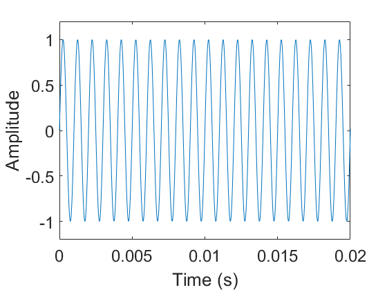
The figure below shows a sinusoidal acoustic signal with a frequency of 1 kHz. The horizontal axis represents time, and the vertical axis represents signal amplitude. The amplitude varies periodically between \(1\) and \(-1\), at a frequency of 1 kHz—that is, one thousand complete cycles per second.
To generate this tone, simply run the following MATLAB code. You may use MATLAB’s sound() function (line 5) to play it aloud. At the end, the generated waveform is saved to the local file sound.wav; playback using any standard audio player should yield identical results to direct playback via sound().
Fs = 48000;                             % Sampling frequency (Hz)
T = 4;                                  % Duration (seconds)
f = 1000;                               % Signal frequency (Hz)
y = sin(2*pi*f*(0 : 1/Fs : T));         % Generate tone
sound(y,Fs)                             % Play tone
audiowrite('sound.wav', y, Fs);         % Save tone
This code fully implements acoustic signal generation, transmission (playback), and local file storage. Note the introduction of the concept of sampling, involving two distinct frequencies: the sampling frequency and the signal frequency. Their definitions, interrelationships, and distinctions will be elaborated in subsequent sections.
Much of the code in this material is written in MATLAB. If you are unfamiliar with MATLAB, refer to the appendix for introductory guidance; numerous additional online resources are also available.
MATLAB can similarly implement acoustic signal reception, as shown in the following code:
Fs = 48000;                             % Sampling frequency (Hz)
Rec = audiorecorder(Fs, 16, 1);         % Define audio recorder object
T = 4;                                  % Recording duration (seconds)
record(Rec, T);                         % Start recording
pause(T);                               % Wait for recording to complete
y = getaudiodata(Rec);                  % Extract recorded audio data
audiowrite('sound.wav', y, Fs);         % Save audio
This code records an acoustic signal for a specified duration and saves it to a local file. During initialization of the recording object, the audiorecorder function is invoked with three parameters—in order: sampling frequency, bit depth (quantization resolution), and number of channels. Understanding this function requires familiarity with key signal processing concepts—including sampling and quantization. In this example, the sampling frequency is set to 48 kHz, the bit depth to \(16\) bits, and the number of channels to \(1\) (i.e., mono). These three parameters jointly define the format of the acquired acoustic signal along three orthogonal dimensions. The number of channels generally indicates how many independent signal paths are captured (e.g., how many microphones were used). In MATLAB, if the number of channels is 1, the recorded audio data is returned as a column vector; if it is 2, the result is a matrix composed of two column vectors—each representing the output of one microphone. A microphone serves as the physical sampling device for acoustic signals; analogously, in electromagnetic wave applications, dedicated electromagnetic sampling hardware (e.g., antennas and RF front-ends) performs signal acquisition.
This constitutes the foundational framework for signal transmission and reception. We encourage all learners to perform these experiments hands-on. This section establishes the acoustic-signal-based simulation of signal transmission and reception. On actual wireless signal platforms, the underlying process is fundamentally similar—only the hardware used for transmission and sampling differs. Using acoustic signals here provides greater intuitiveness and accessibility.