Ranging Based on Signal Propagation Time
Ranging based on signal strength is highly susceptible to environmental influences, often resulting in large errors and is rarely used in real-world systems. In practical applications, ranging based on signal propagation time—commonly known as Time of Flight (ToF)—is more widely adopted.
Signal propagation time, or Time of Flight (ToF), refers to the time a signal takes to travel through a medium. If the propagation speed of the signal in the medium is known, the distance traveled by the signal can be estimated using ToF.
Principle of ToF Ranging
This section introduces common ToF measurement methods, which can serve as a reference when reading research papers or implementing such techniques.
Synchronized Measurement Method
If the transmitter and receiver are precisely time-synchronized, the time it takes for a packet sent from the transmitter to reach the receiver can be accurately measured by recording the exact transmission and reception timestamps. Specifically, under synchronized clocks, the receiver can record the moment the transmitter begins transmission; upon receiving the signal, it immediately records the arrival timestamp; finally, subtracting the transmission time from the reception time yields the signal's flight time.
Let \(d\) denote the distance from transmitter to receiver, \(c\) the signal propagation speed (e.g., speed of sound), and \(t\) the measured flight time. Then we have:
However, two critical challenges arise: first, precise time synchronization between transmitter and receiver is required; second, accurate measurement of transmission and reception times is difficult. These issues make clock synchronization a key challenge in ToF-based ranging.
Traditional networking research has proposed various time synchronization mechanisms. For example, the Network Time Protocol (NTP) serves as the standard for internet time synchronization. Additionally, Global Positioning System (GPS) technology provides global time synchronization across devices. GPS achieves this by employing high-precision cesium atomic clocks on satellites, allowing GPS receivers to synchronize with satellite clocks by decoding pseudorandom sequences transmitted from satellites.
Existing synchronization methods still face significant limitations in practice. NTP is primarily designed for static networks and requires frequent message exchanges to correct frequency offset errors. Moreover, its millisecond-level accuracy is insufficient for high-precision ranging applications. While GPS offers nanosecond-level synchronization precision, it is heavily affected by environmental obstructions and only works reliably in open outdoor environments, making it unsuitable for indoor, low-power IoT nodes.
Due to the difficulty of synchronizing clocks between transmitters and receivers, some approaches integrate both functions into a single device to avoid inter-device clock synchronization when calculating ToF.
The first approach uses the target object as a reflector that directly reflects the transmitted signal. This method requires the reflector to have sufficient size and the transceiver to operate in full-duplex mode—simultaneously transmitting and receiving signals. For instance, Frequency Modulated Continuous Wave (FMCW) signals can be used to measure ToF.
The second approach involves two separate devices acting as transmitter and receiver: the transmitter sends a signal at time \(𝑡_0\), the receiver waits for a duration \(\Delta 𝑡\) after reception before sending back an identical waveform, and the original transmitter records the reply arrival time \(𝑡_1\). The distance is then calculated as: \(𝑑=(𝑣(t_1-t_0-\Delta t))/2\). This method does not require clock synchronization between the two devices nor full-duplex capability.
In essence, the two devices achieve implicit synchronization through data exchange. However, due to unpredictable software/hardware scheduling delays and other factors, the receiver cannot precisely control the waiting time to exactly \(\Delta t\), leading to inaccurate timing and thus significant ranging errors.
Measuring Distance Using Reflected Signals
Frequency Modulated Continuous Wave (FMCW) is a technique widely used in high-precision radar ranging. FMCW signals are characterized by frequencies that change linearly over time. FMCW has a long history and broad application scope. In recent years, it has been increasingly applied in IoT localization and sensing scenarios. Many cutting-edge research works leverage electromagnetic or acoustic FMCW signals for positioning and perception tasks.
One direct application of FMCW is measuring ToF via the frequency difference obtained by mixing the reflected signal with the transmitted signal.
As shown in the solid line in the figure below, an FMCW radar modulates its signal into a specially designed FMCW waveform (similar to the LoRa chirp signal introduced in the LoRa chapter), whose frequency periodically increases (from \(f_{min}\) to \(f_{max}\)) or decreases (from \(f_{max}\) to \(f_{min}\)). An increasing FMCW signal \(R(t)\) with a frequency sweep period \(T\) can be expressed as:
where \(B=f_{max}– f_{min}\) denotes the bandwidth of the frequency sweep.
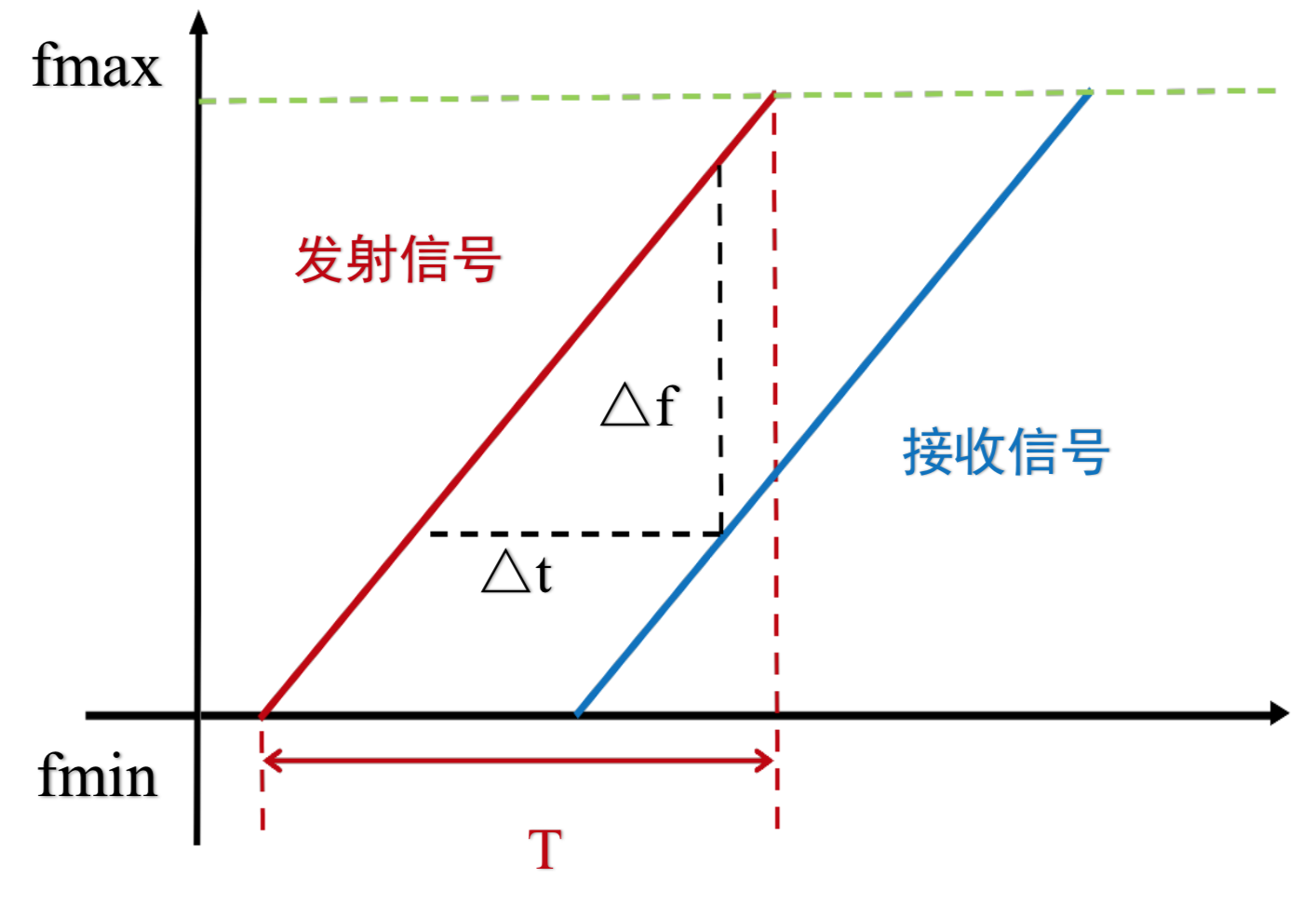
During each sweep cycle, the FMCW radar transmits a continuous wave with varying frequency. The echo reflected from an object is received and superimposed with the transmitted signal. The received signal exhibits a time delay relative to the transmitted one, as illustrated in the figure. Directly measuring this small time delay is challenging in practice (though some studies attempt to do so). To address this, the time delay is converted into a measurable frequency difference—the core advantage of FMCW.
The beat frequency (difference frequency) is relatively low and proportional to the target distance, typically in the kHz range, making it easy to process with hardware and suitable for digital signal processing. Therefore, this method offers advantages such as simplicity, compact structure, lightweight design, low cost, and strong applicability.
Since the frequency difference \(\Delta f\) between the reflected and original signals has a linear relationship with the signal propagation time \(\Delta t\), ToF measurement can be transformed into a frequency measurement. Assuming the distance between the receiver and transmitter is \(d\), and noting that the propagation time \(\Delta t\) represents the round-trip duration, we obtain:
Meanwhile, based on the triangular relationship in the diagram:
Combining these equations, the distance \(d\) can be computed as:
How can we compute the frequency difference? Recall the LoRa decoding process, where computing the starting frequency of a signal is essential. Given a decoding window containing multiple FMCW signals, if we can determine the starting frequency of each, we can derive their frequency difference.
?? Supplement ?? With this foundation, we can simulate radar functionality using smartphones. Leveraging prior knowledge, we can use a smartphone to transmit an FMCW signal while simultaneously recording the reflected acoustic signal, followed by post-processing of the recorded audio.
Single-Sided Two-Way Ranging (SS-TWR)
Single-Sided Two-Way Ranging (SS-TWR) is a ranging method initiated unilaterally using round-trip communication. For clarity, consider two devices \(A\) and \(B\). The timing sequence and packet format of SS-TWR are illustrated below:
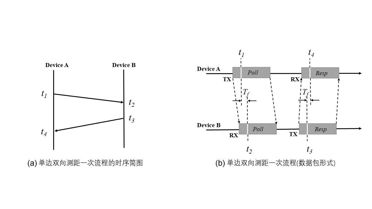
As shown, communication is initiated by device \(A\). At time \(t_1\), \(A\) sends a \(Poll\) packet to \(B\). \(B\) receives the \(Poll\) packet at time \(t_2\), then transmits a \(Resp\) packet back to \(A\) at time \(t_3\), and finally \(A\) receives the \(Resp\) packet at time \(t_4\).
The ToF estimation is straightforward and intuitive. Denoting the measured ToF as \(T_f\), we have:
Error Analysis: Assume the primary source of error is hardware clock drift. We model the clocks of devices \(A\) and \(B\) as follows [2]:
where \(e_a\) and \(e_b\) represent the clock offsets of devices \(A\) and \(B\), respectively. Substituting \(\hat{t}_a\) and \(\hat{t}_b\) into \(T_f\), the ToF considering clock offsets becomes:
Thus, the error is:
Assuming \(T_f= 100 ns\), hence \(t_3-t_2 \approx 1 ms\), and a typical clock drift of \(20ppm\), the error is approximately \(20 ns\), corresponding to a ranging error of \(6m\). From this analysis, we see that the main error in SS-TWR stems from clock drifts between the two devices. Double-Sided Two-Way Ranging (DS-TWR) improves upon this.
Double-Sided Two-Way Ranging (DS-TWR)
Double-Sided Two-Way Ranging (DS-TWR) extends SS-TWR by adding an additional round of communication. Consider two devices \(A\) and \(B\) to illustrate the DS-TWR process:
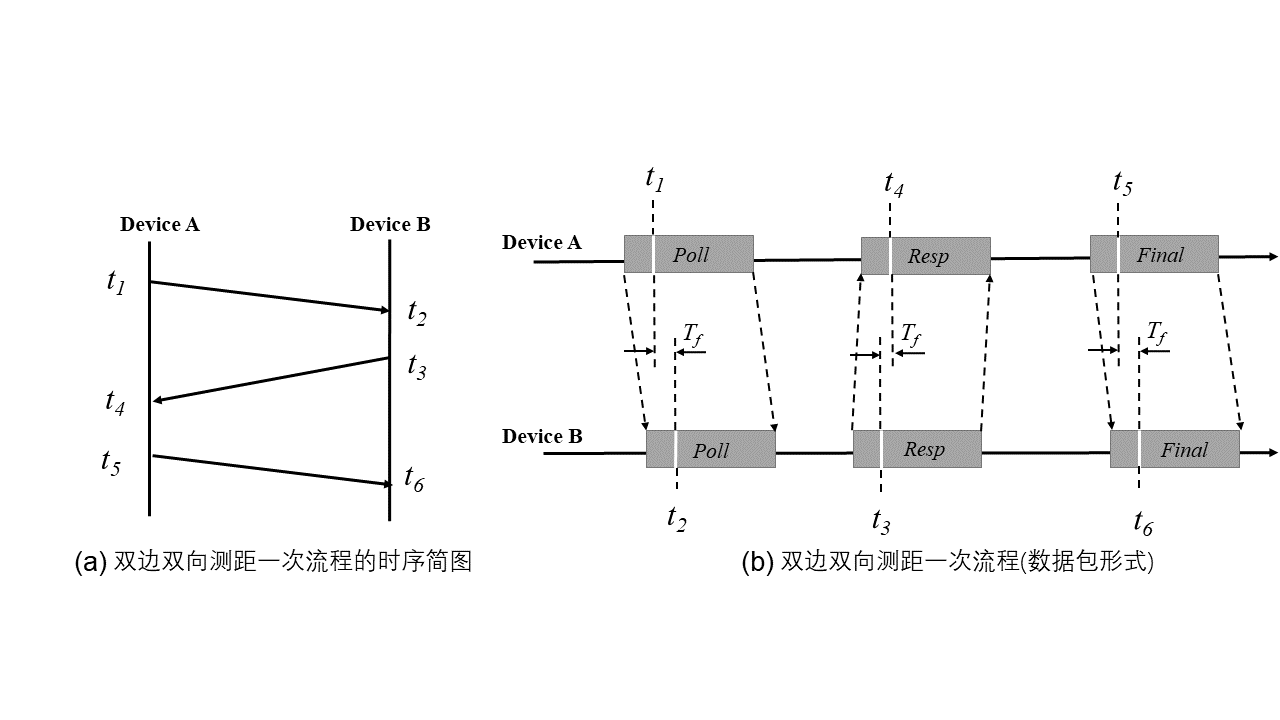
As shown, device \(A\) transmits a \(Poll\) packet to \(B\) at time \(t_1\). Device \(B\) receives it at \(t_2\), replies with a \(Resp\) packet at \(t_3\), and \(A\) receives the reply at \(t_4\)—this completes one SS-TWR cycle. Subsequently, \(A\) sends another \(Final\) packet to \(B\) at \(t_5\), which \(B\) receives at \(t_6\). With this, the DS-TWR process concludes.
Similarly, the ToF \(ToF\) can be calculated as:
Error Analysis: Let us examine why DS-TWR performs better than SS-TWR. Again assuming clock drift as the dominant error source, we model the clocks of devices \(A\) and \(B\) as follows [2]:
where \(e_a\) and \(e_b\) are the clock offsets of devices \(A\) and \(B\), respectively. Substituting \(\hat{t}_a,\hat{t}_b\) into \(T_f\), the ToF considering clock offsets becomes:
Hence, the error is:
Assuming \(T_f= 100 ns\), e.g., for Decawave’s DW1000 chip, \(((t_3-t_2)-(t_5-t_4)) \in (0ns,8ns)\), taking worst-case scenario \(8ns\), with a clock drift of \(20ppm\), the error is approximately \(2 ps\), corresponding to a ranging error of \(0.6mm\). Clearly, DS-TWR offers significantly higher theoretical accuracy than SS-TWR.
Moreover, although the above calculation remains affected by clock drifts from both devices, optimized algorithms can eliminate the influence of one device’s clock, which is why DS-TWR is considered to implicitly achieve time synchronization compared to SS-TWR.
Ranging Using Wave Velocity Difference
In practical systems, if two different types of signals can be used, ranging can also be achieved by exploiting the velocity difference between them.
For example, the transmitter may simultaneously send an electromagnetic wave and a sound wave, and the receiver records the arrival times \(𝑡_𝑟\) (for EM wave) and \(𝑡_𝑠\) (for sound wave). The distance between transmitter and receiver can then be calculated as:
Since \(𝑣_𝑟=3\times 10^8 m/s\) is much greater than \(𝑣_𝑠=340m/s\), the distance formula simplifies to:
\(𝑑=𝑣_𝑠\times (𝑡_𝑠-𝑡_𝑟)\)
Ranging Examples
Most real-world ranging systems are based on the principles outlined above. Later chapters of this book will present several ranging system examples and actual code implementations, including the acoustic BeepBeep ranging method using COTS mobile devices [1] and WiFi Fine Timing Measurement (FTM) protocol [3].
References
[1] Peng, Chunyi & Shen, Guobin & Zhang, Yongguang & Li, Yanlin & Tan Kun. (2007). BeepBeep: A high accuracy acoustic ranging system using COTS mobile devices. SenSys. 1-14. 10.1145/1322263.1322265.
[2] Dries Neirynck, Eric Luk, and Michael McLaughlin. 2016. An alternative double-sided two-way ranging method. In 2016 13th Workshop on Positioning, Navigation and Communications (WPNC). IEEE, 1–4.
[3] "IEEE Standard for Information technology–Telecommunications and information exchange between systems Local and metropolitan area networks–Specific requirements - Part 11: Wireless LAN Medium Access Control (MAC) and Physical Layer (PHY) Specifications". "IEEE Std 802.11-2016 (Revision of IEEE Std 802.11-2012)", pages 1–3534, Dec 2016.
[4] Linsong Cheng, Zhao Wang, Yunting Zhang, Weiyi Wang, Weimin Xu, Jiliang Wang. "Towards Single Source based Acoustic Localization", IEEE INFOCOM 2020.
[5] Yunting Zhang, Jiliang Wang, Weiyi Wang, Zhao Wang, Yunhao Liu. "Vernier: Accurate and Fast Acoustic Motion Tracking Using Mobile Devices", IEEE INFOCOM 2018.