Trilateration Algorithm
Based on distance measurements, it is possible to determine the position of a device or person. In this section, we introduce the trilateration algorithm, which enables us to compute the location of a target device from measured distances.
Fundamental Principle of Trilateration
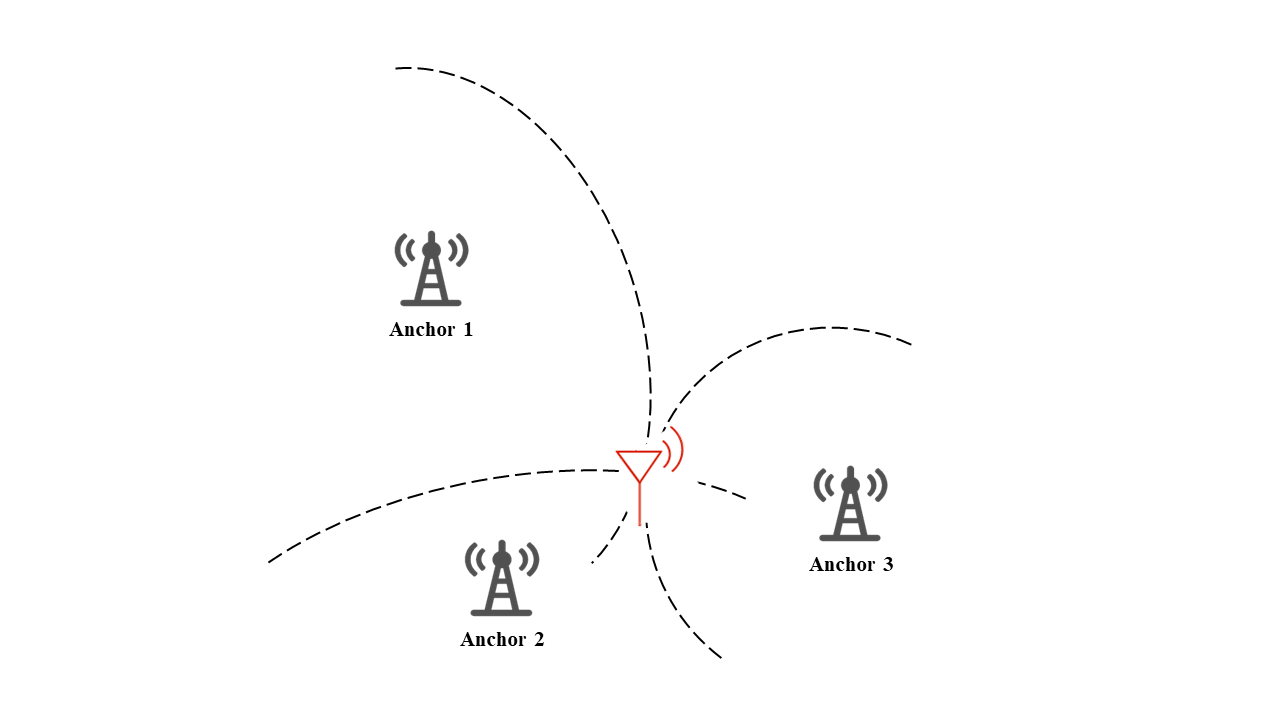
The fundamental principle of the trilateration algorithm is illustrated in the figure below. Suppose we wish to locate the electronic tag (red antenna) shown in the figure, and the positions of all base stations are known. Before computing the tag’s position, we first obtain the distances from each base station to the tag using the ranging methods introduced in the previous chapter: \(d_i\). Based on these ranging results, we draw circles centered at each base station with radii equal to \(d_i\). By searching for the intersection point(s) of these circles in space, we can ultimately determine the tag’s position. The figure below demonstrates how the tag’s location is obtained by computing the common intersection point of three circles, given the coordinates of base stations 1, 2, and 3 and the corresponding distances from the tag to each base station.
The process of searching for circle intersections in trilateration is mathematically equivalent to solving a system of equations. Assume the coordinates of the three base stations are known and denoted as \((x_1,y_1)\), \((x_2,y_2)\), and \((x_3,y_3)\), respectively. Let the unknown coordinates of the target tag be \((x,y)\), and let the measured distances from the tag to the three gateways be \(d_1\), \(d_2\), and \(d_3\), respectively. Then the following system of equations can be formulated:
Solving this system yields the tag’s coordinates. This trilateration algorithm can be straightforwardly extended to three-dimensional scenarios. For 3D localization, after measuring the distances from base stations to the node, we model each base station as the center of a sphere with radius \(d\). The tag must lie somewhere on the surface of each such sphere. Therefore, determining the unique intersection point of multiple spheres yields the tag’s 3D spatial position.
Trilateration is conceptually simple and remains the most widely used localization algorithm. However, practical implementation still faces numerous difficulties and challenges. Due to ranging errors, the circles (or spheres, in 3D) drawn around different base stations may not intersect at a single point. In practice, ranging algorithms yield distance estimates only within a certain error bound. Thus, given a base station’s position, we can typically only assume that the tag lies within an annular region centered at that base station, with some finite radial width. Consequently, designing a coordinate computation method that minimizes localization error becomes an essential consideration during real-world system deployment.
Moreover, in practical environments, the number of base stations may exceed three. When the number of base stations exceeds the dimensionality of the coordinate space, selecting the optimal subset of base stations becomes another critical problem that must be addressed during localization.
In practice, to mitigate the impact of ranging errors on localization accuracy, we commonly employ the least-squares optimization method to solve for the target tag’s coordinates. Suppose the known coordinates of the base stations are \(P_{ai} \ (i=1,2,3...N)\), and let \(N\) denote the total number of base stations. Let the unknown tag coordinates be \(P_t\). Then the theoretical distances from the tag to each base station can be computed as \(d_i\):
Meanwhile, the measured distances from the tag to each base station are known as \(\hat{d}_{i}\). Using this information, we select the position \(P\) that minimizes the difference between theoretical and measured distances as the final localization result:
Below, we present an example solution approach for the above optimization problem. Since the tag position \((x, y)\) lies at the intersection of circles centered at base station positions \((x_i,y_i)\), and the measured distances from the tag to the respective base stations are \(d_i\), a basic approach would be to directly solve the following system of equations (for \(n\) base stations) to obtain the tag coordinates:
However, due to measurement errors, the circles centered at the base stations will generally not intersect at a single exact point. Therefore, an approximate solution must be computed. Common approaches include weighted methods, least-squares methods, and centroid-based methods. Here, we adopt the least-squares method. Starting from Equation (8), we subtract the \(n\)-th equation from each of the first \(n-1\) equations to obtain a linearized system: \(AX=b\), where:
The least-squares solution is then given by:
The MATLAB implementation of the above least-squares solution is as follows:
nodeNumber = 3;   % Number of anchor nodes
nodeList = [0, 0; 2, 0; 1, 1.732];   % Coordinates of three anchor nodes
disList = [1.155, 1.155, 1.155];    % Measured distances from target node to three anchor nodes

A = [];
B = [];
xn = nodeList(nodeNumber, 1);
yn = nodeList(nodeNumber, 2);
dn = disList(nodeNumber);
for i=1:nodeNumber-1
    xi = nodeList(i, 1);
    yi = nodeList(i, 2);
    di = disList(i);
    A = [A; 2 * (xi - xn), 2 * (yi - yn)];
    B = [B; xi * xi + yi *yi - xn * xn - yn * yn + dn * dn - di * di];
end    % Compute parameters A and B for the linear system

X = inv(A'*A)*A'*B   % Compute solution X using the least-squares formula
In the above code, nodeList represents the coordinates of the base stations, nodeNumber denotes the number of base stations, and disList contains the measured distances from the tag to each base station. After computing matrices A and B, the tag’s coordinates X are obtained using Equation (9).
In practical applications, appropriate methods must be selected based on actual conditions. Alternative approaches—beyond least-squares—can be designed to perform approximate position estimation and achieve higher localization accuracy. In certain scenarios, direct analytical solution of the equations may be infeasible or computationally prohibitive; in such cases, numerical approximation methods—such as gradient descent—can be employed.
References
[1] IEEE 802 Working Group et al. 2011. IEEE standard for local and metropolitan area networks—Part 15.4: Low-rate wireless personal area networks (LR-WPANs). IEEE Std 802 (2011), 4–2011.
[2] Dries Neirynck, Eric Luk, and Michael McLaughlin. 2016. An alternative double-sided two-way ranging method. In 2016 13th Workshop on Positioning, Navigation and Communications (WPNC). IEEE, 1–4.
[3] "IEEE Standard for Information technology–Telecommunications and information exchange between systems Local and metropolitan area networks–Specific requirements - Part 11: Wireless LAN Medium Access Control (MAC) and Physical Layer (PHY) Specifications". "IEEE Std 802.11-2016 (Revision of IEEE Std 802.11-2012)", pages 1–3534, Dec 2016.
[4] Benjamin Kempke, Pat Pannuto, Bradford Campbell, and Prabal Dutta. 2016. Surepoint: Exploiting ultra wideband flooding and diversity to provide robust, scalable, high-fidelity indoor localization. In Proceedings of the 14th ACM Conference on Embedded Network Sensor Systems CD-ROM. 137–149.