Distance Measurement Based on Signal Strength
In the Internet of Things (IoT), a commonly required function is measuring the distance between two objects or devices. While traditional methods exist, this material focuses on using inherent capabilities of IoT devices—such as cameras and wireless modules—to perform distance measurement. Specifically, we will introduce methods for distance estimation based on wireless signals.
Definition of Received Signal Strength
Received Signal Strength (RSS), also known as Received Signal Strength Indication (RSSI), is a key metric used in wireless transmission layers to evaluate link quality. The transmission layer uses RSS to determine whether the transmit power should be increased.
Typically, RSS is expressed in terms of power, with the unit watt (W). However, wireless signal energy is generally weak, often at the milliwatt (mW) level. Therefore, it is common practice to represent signal strength logarithmically relative to a reference power of 1 mW, resulting in the unit dBm (decibel-milliwatts). In wireless communications, 1 mW corresponds to 0 dBm; signals weaker than 1 mW have negative RSSI values, while those stronger than 1 mW have positive RSSI values.
Note: \(dB\) is a dimensionless unit, where \(dB = 10\lg X\), allowing extremely large or small numbers to be conveniently represented. In contrast, \(dBm\) represents the ratio of two power levels with a physical dimension (milliwatts), serving as an absolute measure of power. Its calculation formula is: \(10\lg(功率值/1mW)\).
For example: If the transmit power is \(1mW\), its value in \(dBm\) units would be \(10 \lg 1mW/1mW = 0 dBm\); for a power of \(40W\), \(10 \lg(40W/1mW)=46dBm\).
The most commonly used \(2W=33dBm\), \(20W=43dBm\). The difference between \(dBm\) and \(dBm\) can be expressed using \(dB\). For instance, \(46dBm-43dBm=3dB\) indicates that the power \(40W\) is \(2\) times that of \(20W\). Thus, dB provides a convenient way to express relationships between signal levels.
Principle of RSSI-Based Ranging
Intuitively, RSSI is clearly related to distance—the farther the distance, the lower the signal strength.
In the chapter on channel models, we have already analyzed in detail the relationship between signal strength and distance.
Generally, RSSI is influenced by four factors: transmit power, path loss, receive gain, and system processing gain. The formula for received power can be written as:
$$
RSSI = Tx_Power + Path_Loss + Rx_Gain + System_Gain
$$
In the earlier section "Path Loss and Shadowing" from the "Wireless Channel" chapter, we introduced the general model describing how signal strength decreases with distance:
$$
P_{G}=-P_{L}=10 \log {10} \frac{G
$$} \lambda^{2}}{(4 \pi d)^{2}
From this equation, it is evident that if the distance is known, the channel attenuation can be calculated. Conversely, if we can measure both the transmitted and received signal strengths, we can estimate the distance \(d\). However, note that this applies only under ideal conditions. Real-world environments are much more complex, and actual signal strength rarely follows this formula perfectly.
The fading of signals in free space is illustrated below:
Transmit power, receive gain, and system gain are constants. In ideal conditions, path loss is directly related to propagation distance. Therefore, the relationship between transmitted and received power of a wireless signal can be expressed as [1]:
where \(PR\) is the received power, \(PT\) is the transmitted power, \(r\) is the distance between transmitter and receiver, \(c_0\) is a constant related to antenna parameters and signal frequency, and \(n\) is the path loss exponent, whose value depends on the wireless propagation environment (this formula is a far-field approximation and does not hold when \(r\) is very small). Taking the logarithm of both sides yields:
Since the transmit power is known, \(A=10lg(c_0PT)\) can be interpreted as the received power when the signal travels 1 meter. The left-hand side of the above equation, \(10\lg(PR)\), expresses the received power in dBm, so the equation can be rewritten directly as:
In this equation, the constants \(A\) and \(n\) determine the relationship between received signal strength and transmission distance. We now analyze how these two constants affect the distance estimation.
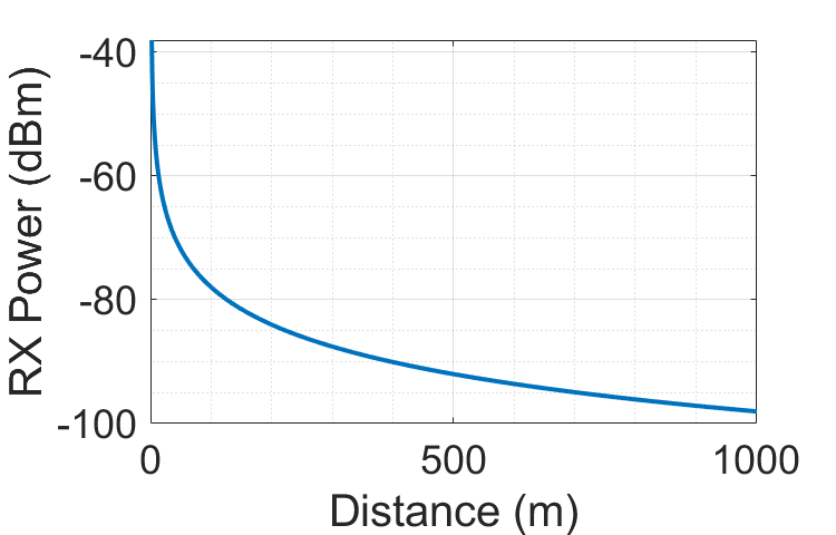
Assuming \(n\) remains constant while varying \(A\), the following relationship curve is obtained:
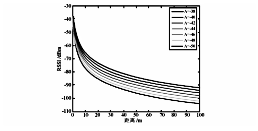
From the figure, we observe that when the path loss exponent \(n\) is constant, the signal strength decays rapidly in the near field but decreases slowly and linearly over long distances. When transmit power increases, the increase in communication range is approximately equal to the ratio of the power increment to the slope of the curve in the flat region. Next, we examine the relationship between RSSI and transmission distance when \(A\) is fixed and different values of \(n\) are used.
As shown in the figure, smaller values of \(n\) result in less signal attenuation during propagation, enabling longer transmission distances. It is also evident that either a favorable path loss exponent (smaller \(n\)) or higher transmit power extends the communication range. The path loss exponent primarily depends on environmental factors such as air attenuation, reflections, and multipath effects. With fewer interferences, \(n\) becomes smaller, the signal propagates farther, and the actual propagation curve approaches the theoretical one, leading to more accurate RSSI-based ranging.
Implementation of RSSI-Based Ranging
To use RSSI for distance estimation, the values of \(A\) and \(n\) must be known in advance. Here, \(A\) denotes the RSSI measured at the receiver when the transmitting and receiving nodes are separated by \(1m\) meters, and \(n\) is the path loss exponent. Both values are empirical and depend on the specific hardware and propagation environment. These parameters must be calibrated within the target application environment before ranging. The accuracy of this calibration directly affects the precision of distance estimation.
Additionally, if the wireless node system operates outdoors, meteorological conditions such as temperature and humidity variations can influence wireless signal transmission. These effects can be mitigated using techniques such as averaging or weighted filtering of consecutive measurements.
To improve ranging accuracy, the instability of RSSI must be minimized so that RSSI values better reflect true transmission distances. Various filters can be designed to smooth RSSI readings. The two most commonly used and easily implemented filters are the mean (average) filter and the weighted filter. The average filter is the most basic form but requires multiple transmissions between sender and receiver to compute a reliable estimate.