AoA Localization Algorithm

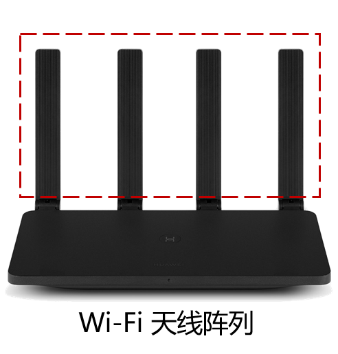
Angle of Arrival (AoA)–based localization is a common wireless positioning technique and one of the most widely adopted algorithms in practical systems. It also appears frequently in cutting-edge research works. Computing the angle of arrival may sound complex, and many people lack hands-on experience—thus missing an intuitive understanding. The core idea is to use hardware devices to sense the direction from which signals transmitted by other devices arrive, thereby estimating the relative orientation between the receiver and transmitter. This is typically achieved using multi-antenna arrays (Antenna Arrays). Below is an example of a linear Wi-Fi antenna array. By measuring multiple AoA values, the unknown position of a node can be determined via triangulation or similar geometric methods. AoA algorithms are employed extensively in radar technology and state-of-the-art IoT sensing and localization systems.

Figure. Wi-Fi Antenna Array

This section presents the fundamental principles and practical implementation of AoA localization through both theoretical explanation and executable code. In the subsequent chapter “Acoustic Sensing”, we will demonstrate how to implement AoA using real acoustic signals and a multi-microphone array to compute actual channel arrival angles.

Methods for Estimating Angle of Arrival

Estimating AoA generally relies on antenna array techniques. As illustrated below, for signals arriving at a multi-antenna array from different directions, the received signals across individual antennas exhibit time delays. These inter-antenna time differences correspond directly to the signal’s angle of arrival—constituting the foundational principle of AoA estimation. Thus, the central challenge in AoA is accurately estimating the time difference of arrival (TDOA) across antennas. While conceptually straightforward, achieving high accuracy in practice is highly nontrivial.

Common approaches for estimating inter-antenna TDOA include:

Using signal delay estimation techniques—e.g., cross-correlation—to determine the time delays among array-received signals; combining these with signal propagation velocity and array geometry yields AoA information. See the “Acoustic Sensing” chapter for details.
Employing the Multiple Signal Classification (MUSIC) algorithm.
Applying beamforming techniques—commonly known as Beamforming—to enhance signals arriving from specific directions and infer AoA from directional signal strength measurements.

Although these algorithms are widely discussed, few practitioners have implemented them. In this chapter and the following ones, we will guide you step-by-step through their implementation.

Figure. Directional Gain Variation Due to Array Geometry. Source: [1]

MUSIC Algorithm

The Multiple Signal Classification (MUSIC) algorithm is a widely used method for AoA estimation.

?? Yang Zijiang’s analysis section to be added.

The core idea is to perform eigen-decomposition of the covariance matrix of array output data, separating it into a signal subspace (spanned by eigenvectors associated with large eigenvalues) and a noise subspace (spanned by eigenvectors corresponding to small eigenvalues), which is orthogonal to the signal subspace. Exploiting this orthogonality, MUSIC constructs a spatial spectrum function and estimates signal parameters—including incident direction, polarization, and power—by searching for spectral peaks.

Assume an equispaced linear antenna array with $N$ antennas, inter-element spacing $d$, and signal wavelength $\lambda$. Suppose there are $r$ signal sources in space. The received signal vector can be expressed as
$$ X\left(t\right)=\sum_{i=1}^{r}{s_i\left(t\right)a\left(\theta_i\right)}+N\left(t\right) $$
where $s_i(t)$ denotes the signal from the $i$-th source, $\theta_i$ is the incident angle of the $i$-th source, and $A(\theta_i)$ is given by
$$ a\left(\theta_i\right)=\left[1,e^\frac{j2\pi dsin\left(\theta_i\right)}{\lambda},\ldots,e^\frac{j2\pi\left(N-1\right)dsin\left(\theta_i\right)}{\lambda}\ \right]^T $$
The received signal vector is then
$$ X\left(t\right)=AS\left(t\right)+N\left(t\right) $$
where $A=[a\left(\theta_1\right),a\left(\theta_2\right),\ldots,a(\theta_r)]$ and $S(t)=\left[s_1\left(t\right),s_2\left(t\right),\ldots,s_r\left(t\right)\right]^T$.

The covariance matrix of $X\left(t\right)$ is
$$ R_X=E\left[XX^H\right] $$
with $X^H$ denoting the conjugate transpose of $X$. Assuming uncorrelated zero-mean white noise, we obtain
$$ R_X=E\left[\left(AS+N\right)\left(AS+N\right)^H\right]=AE\left[{SS}^H\right]A^H+E\left[NN^H\right]={AR}_SA^H+R_N $$
where $R_S=E[SS^H]$ is the signal correlation matrix, $R_N=\sigma^2I$ is the noise correlation matrix, and $\sigma^2$ is the noise power.

Performing eigen-decomposition on the array covariance matrix, first consider the noiseless case. For matrix $A$, if the $r$ signal sources have distinct incident angles and $N>r$, then the columns of $A$ are linearly independent, and $AR_SA^H$ has rank $r$. Since $R_S^H$ = $R_S$ and $R_S$ is positive definite, ${AR}_SA^H$ is positive semi-definite, possessing $r$ positive eigenvalues and $N-r$ zero eigenvalues.

In the presence of noise, $R_X=AR_XA^H+\sigma\ I^2$, since $\sigma>0$ and $R_X$ is full-rank, ${AR}_SA^H$ has $N$ positive real eigenvalues: $r$ of them correspond to signal components—equal to the ${AR}_SA^H$ largest eigenvalues of $r$ plus $\sigma^2$—while the remaining $N-r$ smallest eigenvalues $\sigma^2$ correspond to noise.

Let $\lambda_i=\sigma^2$ denote the noise-associated eigenvalues and $v_i$ their corresponding eigenvectors. Then
$$ R_Xv_i=\lambda_iv_i=\sigma^2v_i=\left(AR_SA^H+\sigma^2I\right)v_i $$
Hence
$$ {AR}SA^Hv_i=0 $$
Multiplying both sides by $R_S^{-1}\left(A^HA\right)^{-1}A^H$ yields
$$ A^Hv_i=0,\ i=r+1,\ldots,N $$
Therefore, selecting the $N-r$ eigenvectors associated with the smallest eigenvalues forms the noise subspace matrix $E_n$:
$$ E_n=[v},v_{r+2},{\ldots,vN] $$
Define the spatial spectrum as
$$ P $$}\left(\theta\right)=\frac{1}{a^H\left(\theta\right)E_nE_n^Ha(\theta)}=\frac{1}{\left|\left|E_n^Ha\left(\theta\right)\right|\right|^2
Searching over $\theta$, the angles at which $P_{mu}\left(\theta\right)$ attains its peaks correspond to the directions of the signal sources.

Beamforming Algorithms

Beamforming leverages antenna arrays to enhance signals arriving from specific directions, enabling directional transmission or reception.

Delay-and-Sum Beamforming

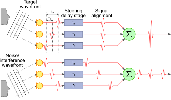
For discrete-time signals, delay-and-sum beamforming provides a simple and direct method for estimating the direction of arrival.

Let $i$ denote the signal received by the $x_i\left(t\right)$-th antenna. To estimate the AoA $\theta$, we sweep over candidate angles, apply angle-dependent time delays $\tau_i(\theta)$ to each antenna’s signal, and sum the delayed signals:
$$ x\left(\theta\right)=\sum_{i=1}^{n}{x_i(t-\tau_i\left(\theta\right))} $$
The direction yielding the maximum summed signal energy is taken as the estimated AoA:
$$ \theta_{AOA}=\text{argmax}_{\theta}{x(\theta)} $$
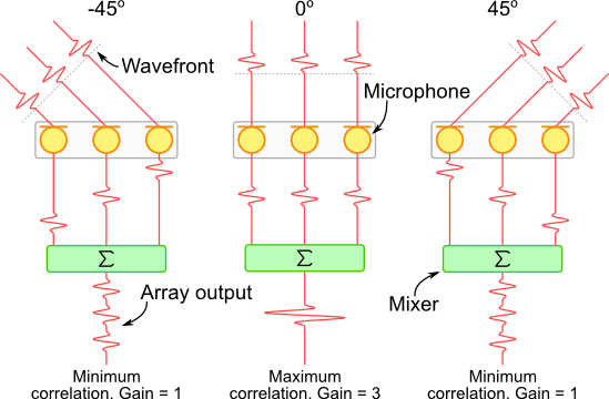
For the three-microphone array shown above, adding a summation module behind the microphones results in direction-dependent gain. As illustrated, signals arriving from −45° and +45° yield unit gain, whereas signals from 0° achieve a gain of 3. Using this principle, discrete signals received by each microphone can be individually delayed—without altering the physical array geometry—to enhance signals from a desired direction.

Figure. Delay-and-Sum Beamforming. Source: [1]

Steered-Response Power (SRP) Beamforming

Steered-Response Power (SRP) is a beamforming algorithm [2] that enhances signals from arbitrary directions via delay-and-sum processing. In 3D localization scenarios, SRP performs a grid search over candidate spatial points (potential source locations), computes the time difference of arrival (TDoA) between each point and the microphone array, applies corresponding delays, and sums the signals. The spatial point producing the highest output acoustic energy is selected as the estimated source location. The core principle of SRP is as follows:

Assume a system with $M$ microphones indexed by $m\in \{1,...,M\}$, receiving discrete-time signals $s_m(n)$. For a candidate spatial point $x=[x,y,z]^T$, the steered-response power (SRP) is defined as
$$ P(x) = \frac{1}{2\pi}\sum_{m_1=1}^M \sum_{m_2=1}^M \int_{-\pi}^{\pi} S_{m_1}(e^{j\omega})S_{m_2}^*(e^{j\omega})e^{j\omega\tau_{m1,m2}(x)} d\omega $$
where $S_{m}(e^{j\omega})$ is the Fourier-transformed signal, and $\tau_{m1,m2}(x)$ is the TDoA between point $x$ and microphones $m_1$ and $m_2$:
$$ \tau_{m1,m2}(x) = \lfloor f_s \frac{|{x-x_{m_1}}|-|{x-x_{m_2}|}}{c} \rceil $$
Analogous to the Generalized Cross-Correlation (GCC) method, the spatial location $g$ maximizing SRP is taken as the estimated source position:
$$ \hat{x}s = \text{argmax}P(x) $$
With deeper reflection, one recognizes that this computation is essentially equivalent to finding the peak of a cross-correlation function.

SRP with Phase Transform (SRP-PHAT)

Standard SRP exhibits limited robustness against reverberation and noise. DiBiase et al. proposed SRP-PHAT (Steered-Response Power Phase Transform), an enhanced variant applying phase transform—a frequency-domain whitening operation using weighting function $\Phi_{m_1,m_2}(e^{j\omega})$—to improve performance under adverse acoustic conditions. Its conceptual foundation parallels that of GCC-PHAT:
$$ P(x) = \frac{1}{2\pi}\sum_{m_1=1}^M \sum_{m_2=1}^M \int_{-\pi}^{\pi} \Phi_{m_1,m_2}(e^{j\omega})S_{m_1}(e^{j\omega})S_{m_2}^(e^{j\omega})e^{j\omega\tau_{m1,m2}(x)} d\omega $$
$$ \Phi_{m_1,m_2}(e^{j\omega}) = \frac{1}{|{S_{m_1}(e^{j\omega})S_{m_2}^(e^{j\omega})|}} $$

Despite its advantages, SRP-PHAT still faces practical challenges: achieving high localization accuracy requires exhaustive spatial sampling, demanding substantial computational resources—making real-time implementation difficult on resource-constrained devices.

Localization Using AoA Measurements

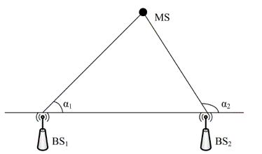
Figure 13-6. Principle of AoA-Based Localization

As shown, the base station (BS) coordinates are known. Signals transmitted from BS arrive at two target nodes with measured AoAs $\alpha1$ and $\alpha 2$. Two rays emanating from the BS, oriented at these respective angles, intersect at the target node. Solving for their intersection yields the node’s position.

Denote the coordinates of BS₁ as $(x_1,y_1)$, BS₂ as $(x_2,y_2)$, and the unknown target node as $(x,y)$.

Assuming neither $\alpha_1$ nor $\alpha_2$ equals $90°$, the equations of the two rays are
$y-y_1=k_1(x-x_1)$ and $y-y_2=k_2(x-x_2)$, where $k_1=\tan(\alpha_1)$ and $k_2=\tan(\alpha_2)$.

Solving for the intersection coordinates:
$$ \left{ \begin{aligned} y-y_1=k_1(x-x_1) \ y-y_2=k_2(x-x_2) \end{aligned} \right. $$
yields
$$ \left {\begin{aligned} &x=\frac{k_1x_1-k_2x_2-y_1+y_2}{k_1-k_2} \ &y=\frac{k_1k_2(x_1-x_2)-k_2y_1+k_1y_2}{k_1-k_2} \end{aligned} \right. $$

Suppose BS₁ = $(0,0)$, BS₂ = $(1,0)$, $\alpha_1=30°$, $\alpha_2=120°$. The MATLAB code for computing the target node’s position (res\AoA_simulation.m) is:

x1=0;y1=0;x2=1;y2=0;
alpha_1=30;alpha_2=120;
k1=tan(alpha_1/180*pi);k2=tan(alpha_2/180*pi);

x=(k1*x1-k2*x2-y1+y2)/(k1-k2)
y=(k1*k2*(x1-x2)-k2*y1+k1*y2)/(k1-k2)

Output:

x = 0.7500
y = 0.4330

$(x,y)=(0.75,0.433)$ is thus the estimated position of the target node.

If either $\alpha_1$ or $\alpha_2$ equals $90°$, the ray equations reduce to $x=x_1$ or $x=x_2$, respectively; solving jointly with the other ray yields the target position.