Doppler Effect-Based Tracking Method
Target Tracking Techniques
The most straightforward approach to target tracking is localization-based: if we can compute the target’s position, continuous tracking becomes trivial by repeatedly calculating its position.
However, localization and tracking impose different requirements. In practical systems, absolute localization of the target is not always necessary to achieve tracking—i.e., estimating the target’s relative motion direction and distance change suffices. Given knowledge of the target’s initial position, continuous tracking and full localization become feasible.
Target tracking techniques exploit signal characteristics (e.g., frequency, phase) that vary during target motion to sense spatial position changes and reconstruct the target’s trajectory. This chapter introduces target tracking using motion-induced distance-change measurements as an example.
Unlike distance-measurement-based localization methods, distance-change-based motion tracking does not directly measure absolute distance; instead, it infers distance change indirectly via associated variations in signal properties such as frequency or phase.
Doppler Effect
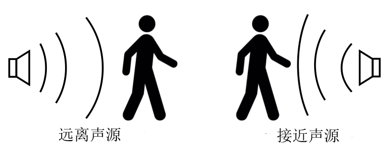
The Doppler effect refers to the phenomenon where the frequency of a received signal differs from the frequency emitted by the source when there is relative motion between the source and the receiver.
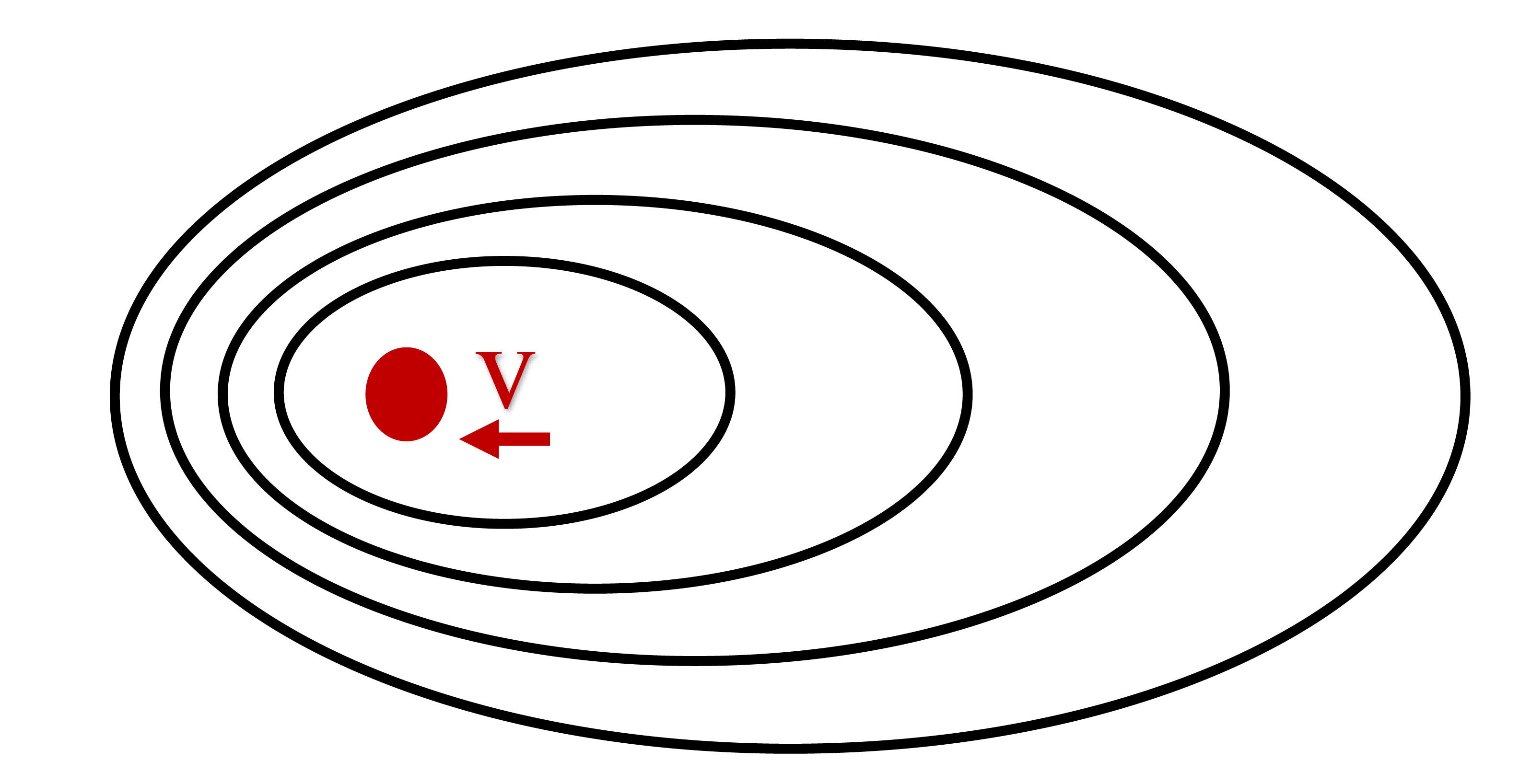
As illustrated, assume the sound source remains stationary while the receiver moves with velocity \(v\). The frequency \(f\) observed by the receiver is given by:
where \(f_0\) denotes the source-emitted frequency, \(c\) denotes the speed of sound, \(v\) denotes the receiver’s speed—positive when moving toward the source and negative when moving away.
Due to the Doppler effect, the received frequency decreases when the receiver recedes from the source and increases when approaching it.
Principle of Doppler-Based Tracking
From the Doppler formula, the receiver’s velocity \(v\) can be derived from the frequency shift between the source and the received signal:
where \(f_0\) is the source-emitted frequency, \(\Delta f\) is the Doppler-induced frequency shift, and \(c\) is the speed of sound.
Since displacement equals the time integral of velocity—i.e., \(d = \int_0^{T} v dt\)—integrating the computed velocity yields the cumulative distance change undergone by the receiver. With knowledge of the receiver’s initial position, its instantaneous position can be determined, thereby enabling target tracking.
The core step in Doppler-based tracking is computing the received signal’s frequency offset \(\Delta f\). To estimate \(\Delta f\), the received acoustic signal is processed using the Short-Time Discrete Fourier Transform (STFT). STFT is a sliding-window-based Fourier transform method: it applies a moving window over the original signal and computes the Fourier transform for each windowed segment, yielding time-localized spectral information. From this, the dominant frequency \(f\) within each time window can be extracted. STFT was introduced in the Fourier Transform chapter; readers are encouraged to revisit that section for review.
If the original signal’s frequency \(f_0\) is constant, the frequency offset \(\Delta f\) is obtained simply as the difference between the original and received frequencies: \(f-f_0\).
Assuming a window length of \(L_w\) samples and a sampling rate of \(f_s\), the frequency resolution \(D_f\) achievable with Doppler-based tracking is given by:
Given the known source frequency \(f_0\) and speed of sound \(c\), the corresponding velocity resolution can be computed as:
Generally, shorter windows yield superior time-domain resolution—enabling finer temporal granularity in frequency estimation—but poorer frequency-domain resolution (i.e., lower frequency discrimination). Conversely, longer windows improve frequency resolution at the expense of temporal resolution.
Implementation of Doppler-Based Tracking
We implement Doppler-based tracking using a single-frequency acoustic signal. The sound source emits a 21 kHz tone. A mobile device records audio while first moving 10 cm away from the source, then an additional 20 cm away, and finally returning to its initial position. The recorded audio file record.wav is analyzed to reconstruct the device’s motion. The implementation code is as follows:
First, a bandpass filter is applied to the received data to suppress noise.
% Read audio file
[data,fs] = audioread('record.wav');
% Extract first channel
data=data(:,1);
% Convert to row vector
data=data.';

% Apply bandpass filter to suppress noise
bp_filter = design(fdesign.bandpass('N,F3dB1,F3dB2',6,20800,21200,fs),'butter');
data = filter(bp_filter,data);
Next, the received signal is processed using STFT with a window length of 1024 samples, zero-padded by a factor of 256 to enhance frequency resolution.
Consider why this zero-padding operation is necessary.
%% Compute frequency offset using STFT
% Window size: 1024 samples
slice_len = 1024;
slice_num = floor(length(data)/slice_len);
delta_t = slice_len/fs;

% Dominant frequency per time window
slice_f=zeros(1,slice_num);
% Zero-pad FFT to 256× resolution
fft_len = 1024*256;
for i = 0:1:slice_num-1
    % Perform FFT on current window; peak frequency in spectrum is taken as window frequency
    fft_out = abs(fft(data(i*slice_len+1:i*slice_len+slice_len),fft_len));
    [~, idx] = max(abs(fft_out(1:round(fft_len/2))));
    slice_f(i+1) = (idx/fft_len)*fs;
end
Finally, the frequency analysis results are used to compute the device’s instantaneous velocity and cumulative displacement per time window, and the resulting distance-vs.-time curve is plotted.
%% Compute distance variation
f0=21000;
c=340;

% Initial position set to zero
position=0;
distance=zeros(0,slice_num);
v = (slice_f-f0)/f0*c;
for i = 1:slice_num
    % Approximate motion within each window as uniform velocity
    % Since positive velocity indicates motion toward the source, distance update uses subtraction
    position = position - v(i)*delta_t;
    distance(i) = position;
end

time = 1:slice_num;
time = time*delta_t;
plot(time,distance);
title('Doppler Effect-Based Tracking');
xlabel('Time (s)');
ylabel('Distance (m)');
The analysis result is shown below:
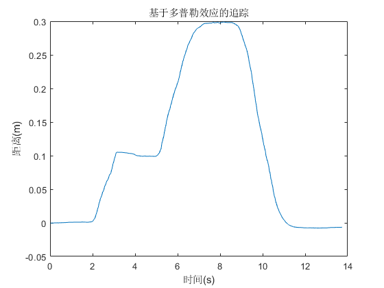
The reconstructed trajectory closely matches the actual motion profile, demonstrating that Doppler-based methods enable accurate motion tracking.