Phase-Based Tracking Methods
Phase-based localization and tracking is a commonly used technique in IoT positioning and tracking. In recent years, a series of phase-based localization and tracking methods have emerged, continuously evolving within the research community. Readers who regularly follow IoT-related academic literature will likely be quite familiar with these approaches. For those wishing to study this topic in depth, it is advisable first to consider the fundamental characteristics of signals themselves—this provides intuitive insight into phase-based tracking methods. Indeed, such methods were proposed long ago; their application in IoT contexts has made their principles more tangible and accessible.
Principle of Phase-Based Tracking
The fundamental principle of phase-based localization is to measure changes in signal phase. Phase was introduced in the chapter on data modulation; readers are encouraged to review that section.
During localization, phase-based tracking can be interpreted from several perspectives.
Assume a signal source emits a continuous-wave (CW) signal of fixed frequency \(R(t)=Acos(2\pi ft)\). This signal propagates along a path of length \(p\), where the path length varies over time as \(d_p(t)\). The received acoustic signal after propagation along path \(p\) can be expressed as:
where \(A_p(t)\) denotes the amplitude of the received signal, \(2\pi fd_p(t)/c\) represents the phase shift induced by propagation, \(c\) is the speed of sound, and \(\theta_p\) denotes a constant phase offset arising from hardware delays, half-wave losses due to reflections, etc.—this term remains invariant over time. If the phase information can be extracted from the received signal \(R_p(t)\), then variations in the propagation path length \(d_p(t)\) can be deduced, thereby enabling trajectory tracking of the receiver.
By employing multiple acoustic sources located at distinct positions and emitting sound waves at different frequencies, and assuming the initial position is known, the spatial displacement of the device can be computed from its time-varying distances to each source—thus achieving high-precision localization and tracking.
Implementation of Phase-Based Tracking
If you have read this material from the beginning, the term phase should already be familiar. Otherwise, we recommend first reviewing the section on digital signal modulation and demodulation, where phase is explained in detail. After studying that section, you will readily understand how phase is leveraged for tracking—hence the emphasis earlier in this material on foundational topics such as Fourier analysis and modulation/demodulation.
To extract the path length \(d_p(t)\) from the received signal, I/Q modulation and demodulation is employed to eliminate terms containing the carrier frequency \(f\).
Given that
multiplying the received signal \(R_p(t)\) by \(\cos(2\pi ft)\) yields a composite signal comprising low-frequency and high-frequency components. Passing this result through a low-pass filter isolates the low-frequency component, termed the in-phase (I) channel signal: \(I_p(t)=\frac{A_p(t)}{2}\cos(2\pi f \frac{d_p(t)}{c}+\theta_p)\). Similarly,
multiplying the received signal \(R_p(t)\) by \(\sin(2\pi ft)\) and applying a low-pass filter yields the quadrature (Q) channel signal: \(Q_p(t)=\frac{A_p(t)}{2}\sin(2\pi f \frac{d_p(t)}{c}+\theta_p)\).
From \(I_p(t)\) and \(Q_p(t)\), the instantaneous phase \(2\pi f\frac{d_p(t)}{c}+\phi_p=\arctan(\frac{Q_p(t)}{I_p(t)})\) can be computed, thereby yielding the propagation path length \(d_p(t)\).
The concrete implementation code is as follows:
% Read audio file
[data,fs] = audioread('record.wav');
% Extract first channel
data=data(:,1);
% Convert data to row vector
data=data.';
% Apply bandpass filtering for noise suppression
bp_filter = design(fdesign.bandpass('N,F3dB1,F3dB2',6,20800,21200,fs),'butter');
data = filter(bp_filter,data);
%% Compute phase variation
f0=21000;
c=340;
time = length(data) /fs;
t=0:1/fs:time-1/fs;
% Multiply original signal with cosine and sine carriers
cos_wave = cos(2*pi*f0*t);
sin_wave = sin(2*pi*f0*t);
r1=data.*cos_wave;
r2=data.*sin_wave;
% Pass resulting signals through low-pass filter to obtain I and Q components
lp_filter = design(fdesign.lowpass('N,F3dB',6,200,fs),'butter');
I = filter(lp_filter,r1);
Q = filter(lp_filter,r2);
% Compute arctangent to obtain phase
phase=atan(Q./I);
%% Compute distance variation from phase change
% Remove phase discontinuities introduced by arctangent wrapping
phase = phase / pi;
p_difference = phase(2:length(phase))-phase(1:length(phase)-1);
bias =0;
for i = 1:length(p_difference)
if p_difference(i)>0.2
bias=bias-1;
end
if p_difference(i)<-0.2
bias=bias+1;
end
phase(i+1)=phase(i+1)+bias;
end
phase = phase * pi;
distance = phase /(2*pi*f0) *c;
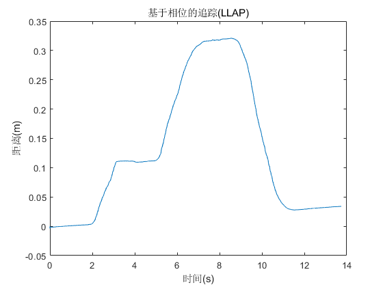
plot(t,distance);
title('Phase-Based Tracking (LLAP)');
xlabel('Time (s)');
ylabel('Distance (m)');
Using the previously described experimental setup, the device first moves 10 cm away from the acoustic source, then an additional 20 cm farther away, and finally returns to its initial position. The tracking result is shown below.
As evident from the result, this method achieves relatively accurate tracking performance.