Acoustic Localization
Building upon the distance measurement techniques introduced earlier, it is natural to extend acoustic methods to localization—simply by applying the trilateration algorithm described previously. We will not elaborate further on this approach here; interested readers are encouraged to experiment with localization performance based on their own distance measurements.
In this section, we focus primarily on Angle-of-Arrival (AoA)-based acoustic localization algorithms.
AoA-Based Localization: Sound Source Localization Using Microphone Arrays
This section introduces sound source localization using linear microphone arrays as an example. By leveraging microphone arrays and the AoA principle, indoor sound source localization can be achieved. First, let us define what a microphone array is.
Microphone Array
The microphone array forms the foundation of AoA-based localization algorithms and serves a function analogous to the antenna arrays discussed in earlier theoretical sections. A microphone array consists of multiple microphones arranged in a specific geometric configuration. Common configurations include linear, rectangular, and hexagonal arrangements. Microphone arrays find broad application in sound source localization, noise suppression, and speech extraction.
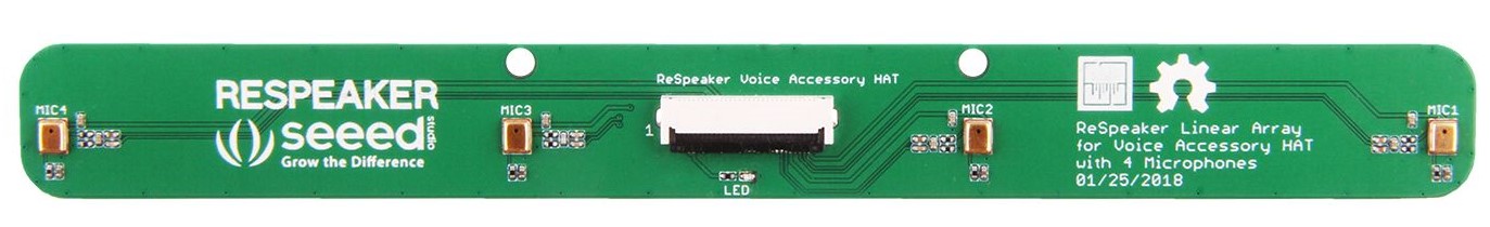
The figure above shows a linear microphone array board with four microphones (the golden components in the image), equally spaced along a straight line. Assuming the sound source is sufficiently far from the array, incident sound waves may be approximated as plane waves. The acoustic propagation model is illustrated below:

As shown, the spacing between two adjacent microphones is \(d\); the angle of arrival (AoA) of the acoustic wave is \(\theta\); thus, the path-length difference from the source to the two microphones is \(d\cos\theta\). Consequently, the time difference of arrival (TDOA) between the two microphones is \(d\cos\theta/c\), where \(c\) denotes the speed of sound. Given the known inter-microphone spacing \(d\) and measured TDOA \(\Delta t\), the AoA \(\theta\) can be computed.
Computing Time Difference of Arrival and Angle of Arrival
The cross-correlation function can be used to estimate the TDOA between two acoustic signals. Let \(M_0\) denote the signal received by microphone \(x(t)\), and \(M_1\) denote the signal received by microphone \(y(t)=Ax(t-t_0)\). Suppose the TDOA between \(M_0\) and \(M_1\) is \(t_0\). Then the cross-correlation function between \(x(t)\) and \(y(t)\) is defined as:
where \(\ast\) denotes the convolution operation.
Substituting the expression for \(y(t)\) yields:
When \(t=t_0\), \(\phi_{xy}(t_0)=A\int^{+\infty}_{-\infty}x(\tau)^2d\tau\) attains its \(\phi_{xy}(t)\) maximum value.
In practice, direct computation of \(\phi_{xy}(t)\) is computationally expensive. Instead, using the identity \(\mathcal{F}(x(t)\ast y(-t))=X(\omega)Y^{\ast}(\omega)\), where \(X(\omega)\) and \(Y(\omega)\) represent the Fourier transforms of \(x(t)\) and \(y(t)\), respectively, allows efficient computation.
Computing \(X(\omega)Y^{\ast}(\omega)\) and then applying the inverse Fourier transform yields \(\phi_{xy}(t)\): $$ \phi_{xy}(t)=\int_{0}^{\pi}{X\left(\omega\right)Y^\ast\left(\omega\right)e^{-j\omega t}d\omega} $$ Converting time-domain convolution into frequency-domain multiplication significantly reduces computational cost. Moreover, to mitigate reverberation and noise effects, frequency-domain weighting can be applied; a commonly used weighting function is the PHAT (Phase Transform) weighting: $$ \phi_{PHAT}\left(\omega\right)=\frac{1}{|X\left(\omega\right)Y^\ast\left(\omega\right)|} $$ resulting in the modified cross-correlation function: $$ \phi_{xy}(t)=\int_{0}^{\pi}{\phi_{PHAT}\left(\omega\right)X\left(\omega\right)Y^\ast\left(\omega\right)e^{-j\omega t}d\omega} $$ The TDOA is estimated from the peak location of the cross-correlation function, which is then used in TDOA-based AoA estimation.
In summary, identifying the peak of the cross-correlation function yields the TDOA between two microphones, enabling subsequent calculation of the AoA.
Below is an analysis using real recorded data: a linear 4-microphone array was employed while emitting a sound source at a nominal angle of 45° relative to the array. The concrete implementation code for computing TDOA and AoA is provided below (res\correlation.m):
% Read audio file
[data,fs] = audioread('array_record.wav');
% Transpose data so each row corresponds to one channel
data=data.';
% Extract signals from the first and fourth microphones in the array
x=data(1,:);
y=data(4,:);
% Inter-microphone spacing: 15 cm
d=0.15;
c=340;

% MATLAB's built-in cross-correlation function
%[corr,lags] = xcorr(x,y);

% Manual implementation of cross-correlation for TDOA estimation
X=fft(x);
Y=fft(y);

corelation = ifft(X.*conj(Y));

l=length(corelation);

[m,index] = max(corelation);

if index > floor(length(corelation)/2)
    index = (index-1)-length(corelation);
else
    index = index-1;
end

delta_t = index/fs
% Compute AoA
theta = acos(delta_t*c/d)/pi*180
Result:
delta_t = -3.1250e-04
theta = 135.0995
The computed angle is approximately 135° (supplementary to 45°), consistent with expectations.
By measuring AoA using acoustic signals, modern intelligent devices can perform numerous tasks—for instance, directional audio capture via microphone arrays, determining speaker direction and angle within a room (e.g., smart speakers), enhancing signals from specific angular sectors, and noise suppression.
Sound Source Localization
Using two or more microphone arrays whose positions are known, combined with the measured AoA values, enables sound source localization based on angular information.

As illustrated above, the positions of arrays \(A_1\) and \(A_2\) are known. By estimating the AoAs \(\theta_1\) and \(\theta_2\) of sound emitted from source S, the 2D coordinates of S can be determined. Specific localization procedures follow those outlined in the earlier AoA localization methodology section.
Fingerprint-Based Localization: Sound Source Localization Using Spatial Sound Intensity Distribution
In the theoretical section, we introduced how wireless device localization can be achieved using spatial “fingerprint” features of signal distribution. Analogously, in acoustic systems, localization can be performed using fingerprints derived from the spatial distribution of sound intensity. This section details how such fingerprint-based sound source localization is realized.
First, consider whether sound signals can support fingerprint-based localization. Examining a single-frequency tone emitted by a loudspeaker reveals that different frequencies exhibit distinct radiation patterns: high-frequency tones propagate more directionally, whereas low-frequency tones spread more isotropically. Thus, frequency-dependent propagation characteristics can be exploited for localization.
Existing acoustic localization methods often achieve one-dimensional ranging using only a single loudspeaker and a smartphone. Consider a circular locus at distance L from the loudspeaker: if one-dimensional ranging yields distance L, the smartphone must lie somewhere on this circle. Combining this with the aforementioned spatial intensity distribution property—i.e., received signal strength varies with angular position around the loudspeaker on that circle—enables determination of the smartphone’s angular orientation relative to the loudspeaker, thereby pinpointing its exact location on the circle. This constitutes the fundamental idea behind fingerprint-based smartphone localization using sound intensity.
We simplify the problem of determining the smartphone’s precise location to the following: define a 3×3 grid with side length 15 cm, centered at 30 cm from the loudspeaker; each cell is thus 5 cm × 5 cm. Using acoustic signals, we classify the smartphone’s position into one of these nine cells—reducing the localization task to a 9-class classification problem.
For the acoustic signal, as noted earlier, we select ten sinusoidal tones spanning the common commercial loudspeaker/microphone bandwidth (20 Hz–20 kHz), mix them, and use the composite signal. Concurrently, we implement existing one-dimensional ranging to measure the loudspeaker-to-smartphone distance. After receiving the signal, the smartphone applies bandpass filtering (as described previously) to isolate the ten frequency components and computes their respective intensities \(s_1\ldots s_{10}\). Using the lowest-frequency component’s intensity as reference, the remaining nine intensities are normalized by this reference, yielding nine intensity ratios \(i_1\ldots i_9\). At this stage, we obtain nine intensity ratios plus the loudspeaker-to-smartphone distance—ten parameters in total.
During training, these ten parameters serve as inputs to a single-hidden-layer artificial neural network, while the smartphone’s ground-truth grid cell serves as the target output. The neural network architecture is illustrated in Figure 2-8, where d denotes the loudspeaker-to-smartphone distance, \(i_1\ldots i_m\) represents m intensity ratios (with m = 9 in experiments), and \(p_1\ldots p_n\) denotes the output probabilities across n classes (n = 9, corresponding to the 3×3 grid). During testing, sound signals are acquired at each measurement point, yielding the same nine intensity ratios and distance. These ten parameters are fed into the trained neural network to predict the smartphone’s grid-cell location. Training and test set sampling locations are shown in Figure 2-9: training points consist of four uniformly distributed samples per grid cell; test points consist of three randomly generated coordinates per cell. The neural network outputs a 9-element vector, each element lying in [0,1], representing the probability that the smartphone resides in the corresponding grid cell. The final predicted location is the grid cell associated with the highest probability.
References
- Linsong Cheng, Zhao Wang, Yunting Zhang, Weiyi Wang, Weimin Xu, Jiliang Wang. "Towards Single Source based Acoustic Localization", IEEE INFOCOM 2020. [PDF]
- Yunting Zhang, Jiliang Wang, Weiyi Wang, Zhao Wang, Yunhao Liu. "Vernier: Accurate and Fast Acoustic Motion Tracking Using Mobile Devices", IEEE INFOCOM 2018.
- Pengjing Xie, Jingchao Feng, Zhichao Cao, Jiliang Wang. "GeneWave: Fast Authentication and Key Agreement on Commodity Mobile Devices", IEEE ICNP 2017